
Expected Goals (xG) in NHL Betting
 Available in US

What xG actually tells you
The first NHL season I tracked xG religiously, I learnt a useful lesson about confirmation bias. I had a model that loved a particular team based on their xG differential. They were generating 56% of expected goals in their games — clearly the better side, the model said, regardless of where they sat in the standings. I bet them through the first 30 games and lost steadily. Then I lost more steadily through the next 30. By February, I was 5,000 in the red and the team was sitting comfortably in a playoff spot they had earned through actual goals, not expected ones.
The lesson was not that xG is useless. It is that xG is one input among several, and a punter who treats it as gospel will be punished by variance, finishing skill, goaltender performance and game-state effects that the metric does not capture. Used carefully, xG is a genuinely useful tool. Used naively, it is a faster route to bankroll destruction than not using it at all.
This guide covers what xG actually measures, the gap between xG and real goal differentials, how to find regression candidates, applying xG to totals, and where to source public xG data without paying for institutional feeds.
What xG measures, and what it does not
Expected goals is a model output, not an observation. Public xG models — MoneyPuck, Natural Stat Trick, Evolving-Hockey — take every unblocked shot attempt, code it for location, type (wrist shot, slap shot, deflection, rebound, etc.), score state, situation (even strength, power play, penalty kill), and assign a probability that an average NHL shooter against an average NHL goalie would score from that situation. Sum those probabilities across a game and you get expected goals for each team.
The metric is genuinely useful for evaluating the quality of chances a team is generating and conceding. A team out-shooting their opponent 35-25 might still be losing the xG battle if those 35 shots include a lot of perimeter wristers and the 25 include several high-danger deflections off rebounds. xG corrects for shot quality, which raw shot counts do not.
What xG does not measure is finishing skill, goaltender skill, and luck. A line with three elite shooters will outscore their xG over a season because their conversion rate is genuinely higher than the model’s average shooter assumption. A goaltender having a hot stretch will under-perform xG against (let in fewer goals than expected). And random variance plays a real role — small samples produce gaps between xG and actual goals that nothing about the underlying play can explain.

The gap between xG and real goals
The most useful application of xG in betting is identifying the gap between xG-based expectation and actual results. A team that is creating chances at a top-five rate but sits in the middle of the league for actual goals has either a finishing problem, a goaltending problem against them in the goalie matchups they have faced, or a luck problem. The first two are persistent; the third regresses.
The relevant research finding here ties back to the totals market. The Woodland and Woodland work on hockey totals showed a reverse favourite-longshot bias, with under-bets outperforming closing implied probability in NHL markets. The mechanism is consistent with what xG tells you about most NHL games: actual scoring undershoots expected scoring more often than it overshoots, because elite goaltending and defensive structure suppress finishing rates below the league-average shooter assumption.
What this means for the punter: when xG suggests a high-scoring game ahead, the historical pattern is that actual goals come in lower than the xG model predicts. The market often prices closer to actual scoring trends than to xG trends, which means a punter naively using xG to bet overs is fighting both the books and the historical bias. Used properly, xG is a regression-spotting tool rather than a totals-pricing tool.
Regression candidates from xG
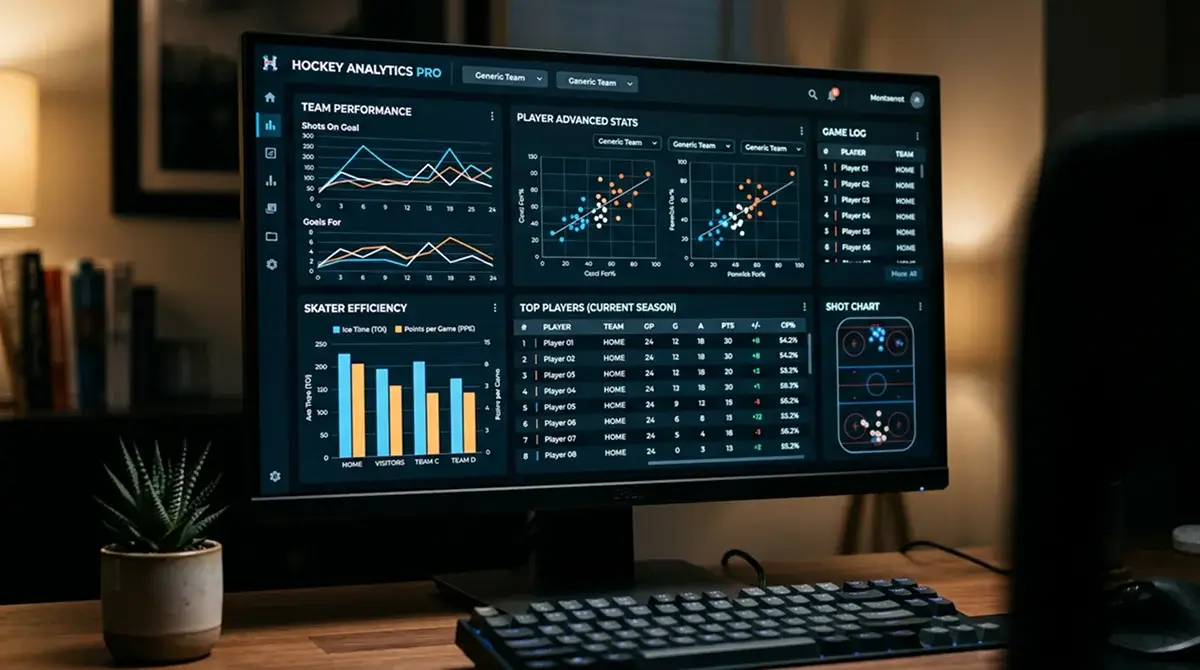
The 1,271 NHL regular-season games (32 teams playing 82 each) provide a long runway to spot regression candidates. By December, the gap between xG and actual goals on most teams has become meaningful enough to evaluate. The thesis: teams whose actual goal differential is materially worse than their xG differential are likely to regress toward their xG over the remainder of the season. The reverse is also true — teams over-performing xG are likely to fall back.
The trickier question is when the regression happens. xG-based regression is not a switch — it is a slow drift over the remaining schedule. Teams that have been unlucky for 30 games might be unlucky for another 30. Books know this and price accordingly: a team with strong xG but poor results often carries a moneyline that already accounts for the expected regression, leaving little edge for a punter who shows up with the same insight a month later than the market did.
The cleanest regression bet is on totals markets rather than match outcomes. A team consistently generating high xG against and conceding low actual goals is a candidate for totals overs in their upcoming games — the goalie regression toward league average produces more conceded goals than the recent record suggests. The same logic applies to props: a player whose shooting percentage is well below career norms but whose xG metrics look stable is a regression-positive prop bet at attractive prices. For the broader framework of treating xG as one input among several in a value betting workflow, the same discipline of finding gaps between model expectation and book pricing applies.

Applying xG to totals
Totals markets are where xG analysis pays back most consistently. The pre-match total reflects the book’s projection of combined goals, which is built from both teams’ offensive xG against expected goalie performance. If your own xG-based projection meaningfully differs from the book’s, you have a thesis worth pricing.
The framework: pull both teams’ even-strength xG-for per 60 minutes and xG-against per 60 minutes from a public source. Adjust for goalie quality on both sides — a top-tier starter suppresses expected goals against by 8-12%, a backup increases them by similar margins. Add in pace expectations (back-to-back fatigue, travel, recent shot-volume trends) and you have a projected game total to compare against the line.
The 6.0 line is the most common, and most pre-match xG projections cluster in the 5.5 to 6.5 range. Meaningful disagreement — a projection of 5.0 or 7.0 — is the signal worth acting on. Marginal disagreement is noise, and the juice will eat any 0.2-goal edge over a long sample.
Where to source public xG data
UK punters do not need to pay for institutional data feeds to use xG effectively. Public xG sources are mature, free, and updated within hours of each game ending. The main options:
MoneyPuck.com publishes team xG, goalie xG, and player-level xG with daily updates. The model is well-documented and the interface is the most user-friendly of the public options. Natural Stat Trick offers more granular filtering — situation, score state, opposition quality — and is the analytical workhorse for deeper dives. Evolving-Hockey publishes the most actively researched models but charges for full access; the free tier is still useful for high-level reads.
The choice between models matters less than consistency. Pick one source and stick with it across a season so your numbers are internally comparable. Jumping between models that use different methodologies (different shot weights, different score-state adjustments) produces noise that drowns out signal. The right discipline is to learn one model deeply rather than sample across several superficially.

The honest use of xG
xG is a tool, not a strategy. Used as the single input to a betting model, it produces consistent losses because finishing variance and goaltender quality dominate short-run outcomes more than expected goals do. Used as one input among several — alongside confirmed starters, line combinations, schedule fatigue, and book pricing — it adds genuine signal to a research workflow.
The discipline is to use xG for regression analysis and totals projection, not for match-outcome prediction. The edge is real but narrow, and the juice will swallow any sloppy application. Used properly, xG is one of the cleaner tradable signals available to UK NHL punters; used carelessly, it is just a fancier way to lose money than not using it at all.
Which public xG model is most stable across NHL teams: MoneyPuck or Natural Stat Trick?
Both are stable and produce highly correlated outputs at the team level. MoneyPuck’s interface is more user-friendly and updates daily with cleaner team-level summaries; Natural Stat Trick offers more granular situation and score-state filtering, which is useful for deeper dives but less digestible at a glance. The choice usually comes down to user preference rather than analytical superiority. The key discipline is to pick one and stay consistent rather than mixing model outputs.
How many games of xG data are needed before betting models trust the signal?
Team-level xG metrics become stable around the 20-25 game mark for offensive xG-for and slightly slower for xG-against, where goalie variance creates additional noise. Player-level xG stabilises later — usually 30-40 games for skaters and 1,500-2,000 shots faced for goalies. Early-season xG carries the same noise problems as early-season Sv%, and any betting model leaning on xG before mid-November is likely working with insufficient sample.
Can xG explain why a hot underdog regresses to the moneyline mean?
Often, yes. A hot underdog whose recent results outstrip their underlying xG performance is a regression candidate, and the moneyline market typically takes a few games to fully reprice the team. The gap between actual goal differential and xG differential is the early warning signal — when the gap widens beyond a couple of goals over a 10-game stretch, regression is statistically likely within the next 10-15 games. Books price slowly enough on mid-season trends that disciplined punters can catch the regression before the market fully adjusts.
Created by the ”ice Hockey Betting” editorial team.